Image Warping - Closed Form Solutions to Homographic and Bilinear Methods

2021/03/09

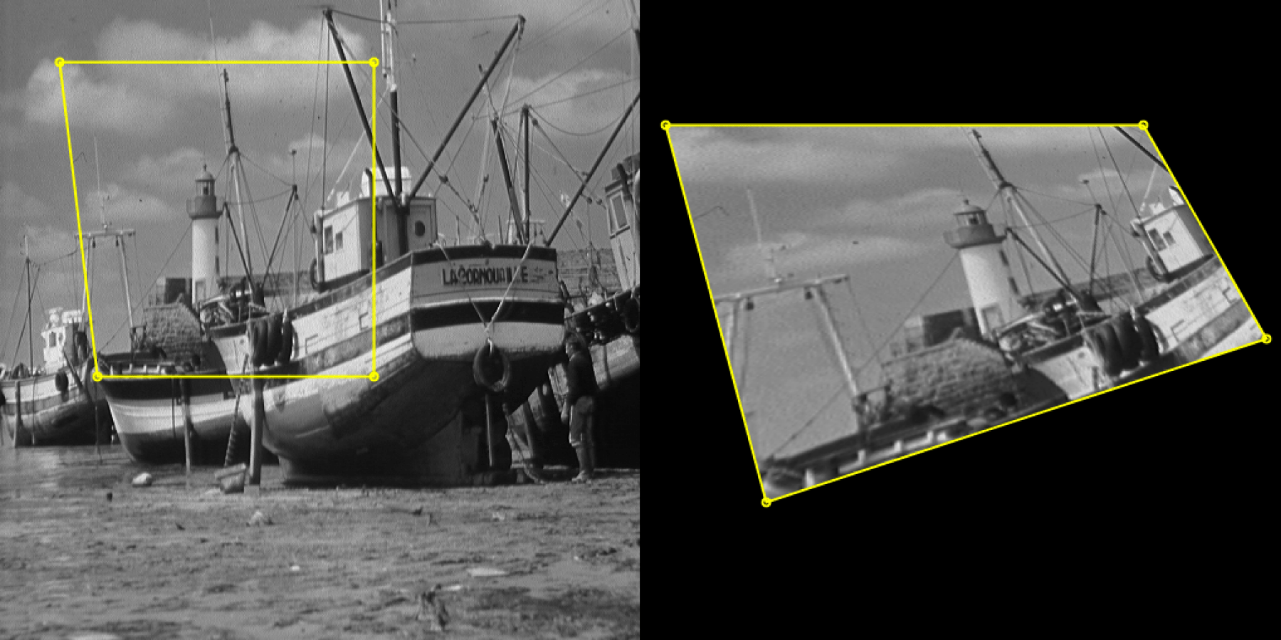
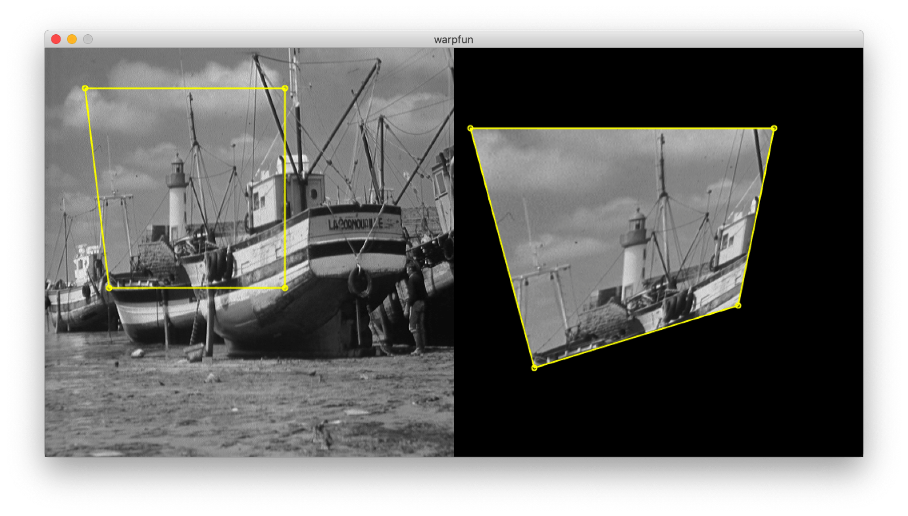
Select 4 points in the source image, and another 4 in the target image. The operation distorts the quadrilateral region from the former to fit into the shape of the latter. This is known as “Warping”. In Photoshop it can be achieved with “distort”. In OpenCV there is a function called warpPerspective.

Perhaps the most common solution to this problem is to use Homography. Homography thinks of the matching points as entities in 3D spaces looked at from different perspectives, and computes a matrix that describes the transform. This is the “correct” model for applications such as straightening out the photo of a document taken at an angle, stitching panoramas, and photoshopping 2D graphics onto an image of a 3D surface.

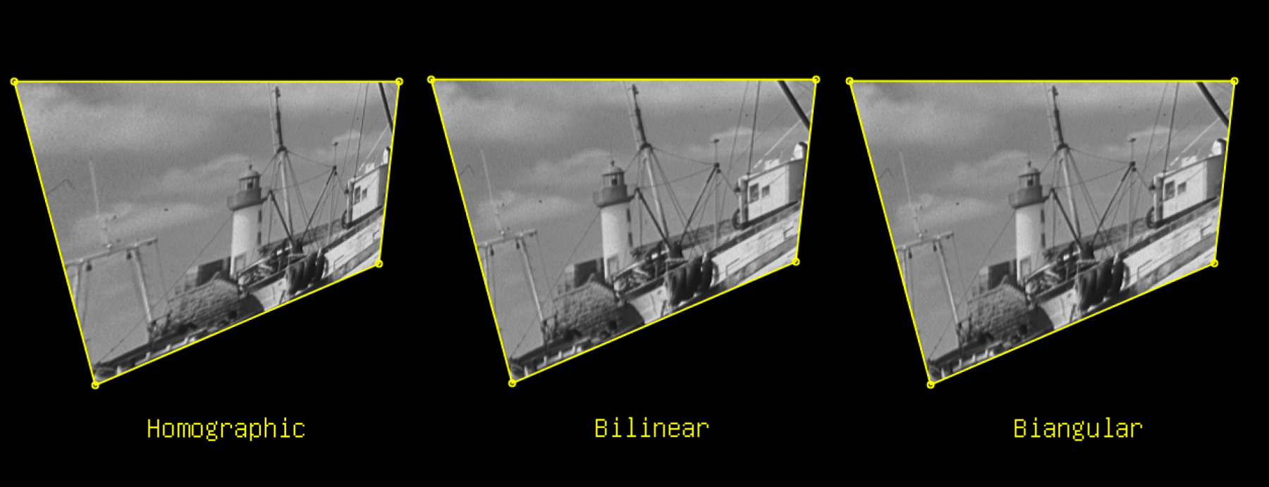
Among other alternatives to homography for warping quads, one can also use bilinear interpolation: Find the bilinear coordinate for each pixel within the target quad (with regard to the quad's 4 vertices), and correspond it to the pixel with the same bilinear coordinate in the source quad. Whereas homography creates a strong perspective effect, the bilinear method gives “flatter” looks.

Tl;dr

I found closed form expressions for these warps (or rather, Mathematica did, at my command). This means that one no longer needs to import packages with linear algebra functionalities such as OpenCV, MATLAB, numpy etc. to solve for each instance of the problem. They can simply substitute the variables into a “magic” formula containing only basic math such as + - * /, trivially portable to any programming environment.

The Java/Processing source code can be found here.

I'm not sure if this has already been done before, but the process of finding these magic formulae had nevertheless been a very fun one for me, so I thought I'd share.

Process

I was re-intrigued by the topic of image warping when reading about it The Pocket Handbook of Image Processing Algorithms in C. The code listing contains in fact the bilinear interpolation warping in disguise -- the introductory text and the way it cleverly pre-calculates invariants led me to initially believe it is solving for a transformation matrix. The original code looks something like this (sans the typos, illustration my own):

//                       
// (sx,sy)                (Wx[0],Wy[0]) +----+ (Wx[1],Wy[1])
//   +------+                          /    /
//   |      |        ->               /    /
//   +------+(ex,ey)   (Wx[3],Wy[3]) +----+ (Wx[2],Wy[2])
void warp(Image Img, Image Out, int sx, int sy, int ex, int ey, int[] Wx, int[] Wy){
  float a,b,c,d,e,f,i,j,x,y,destX,destY;
  float a = (float)(-Wx[0]+Wx[1])/(ey-sy);
  float b = (float)(-Wx[0]+Wx[3])/(ex-sx);
  float c = (float)(Wx[0]-Wx[1]+Wx[2]-Wx[3])/((ey-sy)*(ex-sx));
  float d = (float)Wx[0];

  e = (float)(-Wy[0]+Wy[1])/(ex-sx);
  f = (float)(-Wy[0]+Wy[3])/(ey-sy);
  i = (float)(Wy[0]-Wy[1]+Wy[2]-Wy[3])/((ey-sy)*(ex-sx));
  j = (float)Wy[0];

  for (y = 0; y < ey-sy; y+=0.5){
    for (x = 0; x < ex-sx; x+=0.5){
      destX = a*x + b*y + c*x*y + d;
      destY = e*x + f*y + i*x*y + j;

      Out.Data[(int)(destY)*Out.Cols+(int)destX] = Img.Data[(int)(y+sy)*Img.Cols+(int)(x+sx)];
    }
  }
}

While it's very straightforward and quite efficient, I did notice a couple limitations:

• The transformation maps pixel coordinates from the source image to the destination image, instead of the other way around. Therefore, the pixels in the destination image will be either oversampled or undersampled, with the latter producing serious artifacts (a.k.a holes). To mitigate the issue, the code iterates pixels in half steps (0.5). This only covers up holes for scaling up to 2x, and will be doing duplicate work for shrinking and scaling less than 2x.
• The region in the source image needs to be rectangular and cannot be an arbitrary quad.

Therefore, I couldn't help thinking about the what'd be a more sophisticated solution to the problem.

Then I recalled that there's this cool thing called Homography, which addresses this exact problem. I learned it in the Computer Vision course at CMU (cool course!). Recall how it works:

Let the coordinates of the $nth$ point in the original image be:

And that of the $nth$ matching point of the target image:

All we need to do is to find such a 3x3 transformation matrix, such that for all $n$:

where

(If you have no idea what I'm yapping about, check out transformation matrices and homogeneous coordinates)

With a linear system of 8 unknowns, and each point pair providing two equations, we need a total of 4 pairs of matching points to lock onto a solution. We can apply approximations if we need to satisfy more matching points. But in this particular case of quads, we have the perfect amount, so $n=4$ shall be what we're focusing on for now.

The next question is coming up with a solution to the system. One way is to rewrite it in the form of $Ax=0$.

To do that, we first multiply each row of the square matrix with the column matrix to get an equation. For example, we get this from the first row:

Rearrange:

Which is equivalent of this matrix multiplication:

We do that for all rows to reach the form of this $Ax=0$:

Then the column matrix will be the eigenvector of the left side 9x9 matrix that correspond to the eigenvalue of 0 (for eigenvector $\lambda$ and eigenvalue $v$, $Av=\lambda v$. If $\lambda=0$, then $Av=0$).

Now if you happen to be using a linear algebra package, the work is done. Simply call eig in numpy, eigen in MATLAB, Eigensystem in Mathematica, EigenSolver in Eigen, and so on.

However, not all programming environments come with those, and even when they do, it can be an overkill to import a whole linear algebra library for just warping some photos.

One way is to implement an eigen solver from scratch. That involves computing QR decompositions and reductions to Hessenberg matrices. While it's not ultra-difficult, nor is it trivial to come up with robust implementations, as numerical stability issues can be rather annoying. I know because I've written a linear algebra library myself. You can check out my implementation for these matrix algorithms here.

So I was thinking if a symbolic solution can be computed. Not by me of course, since it'll be a ton of work. But a perfect job for Mathematica!

And thus I spake:

Eigensystem[{
 {-u1, -v1, -1, 0, 0, 0, x1*u1, x1*v1, x1 },
 {0, 0, 0, -u1, -v1, -1, u1*y1, y1*v1, y1 },
 {-u2, -v2, -1, 0, 0, 0, x2*u2, x2*v2, x2 },
 {0, 0, 0, -u2, -v2, -1, u2*y2, y2*v2, y2 },
 {-u3, -v3, -1, 0, 0, 0, x3*u3, x3*v3, x3 },
 {0, 0, 0, -u3, -v3, -1, u3*y3, y3*v3, y3 },
 {-u4, -v4, -1, 0, 0, 0, x4*u4, x4*v4, x4 },
 {0, 0, 0, -u4, -v4, -1, u4*y4, y4*v4, y4 },
 {0, 0, 0, 0, 0, 0, 0, 0, 0}
}]

And Mathematica choked. Hmm… Perhaps it likes this better:

LinearSolve[{
 {-u1, -v1, -1, 0, 0, 0, x1*u1, x1*v1, x1 },
 {0, 0, 0, -u1, -v1, -1, u1*y1, y1*v1, y1 },
 {-u2, -v2, -1, 0, 0, 0, x2*u2, x2*v2, x2 },
 {0, 0, 0, -u2, -v2, -1, u2*y2, y2*v2, y2 },
 {-u3, -v3, -1, 0, 0, 0, x3*u3, x3*v3, x3 },
 {0, 0, 0, -u3, -v3, -1, u3*y3, y3*v3, y3 },
 {-u4, -v4, -1, 0, 0, 0, x4*u4, x4*v4, x4 },
 {0, 0, 0, -u4, -v4, -1, u4*y4, y4*v4, y4 }
}, {0, 0, 0, 0, 0, 0, 0, 0}]

After thinking for a few moments, it spits this out:

{0, 0, 0, 0, 0, 0, 0, 0, 0}

Well thank you so very much Mathematica! Wonder what took you so long to came up with this perfectly correct solution!

I tried again with Solve, which tends to come up with all solutions instead of just one (In fact, LinearSolve can also be made to work by moving the constant term to the right to eliminate a degree of freedom, but in the end the expression given by Solve is shorter so I went with that):

Solve[{
 {-u1, -v1, -1, 0, 0, 0, x1*u1, x1*v1},
 {0, 0, 0, -u1, -v1, -1, u1*y1, y1*v1},
 {-u2, -v2, -1, 0, 0, 0, x2*u2, x2*v2},
 {0, 0, 0, -u2, -v2, -1, u2*y2, y2*v2},
 {-u3, -v3, -1, 0, 0, 0, x3*u3, x3*v3},
 {0, 0, 0, -u3, -v3, -1, u3*y3, y3*v3},
 {-u4, -v4, -1, 0, 0, 0, x4*u4, x4*v4},
 {0, 0, 0, -u4, -v4, -1, u4*y4, y4*v4}}
 .{a,b,c,d,e,f,g,h} == {-x1,-y1,-x2,-y2,-x3,-y3,-x4,-y4},
  {a,b,c,d,e,f,g,h}]

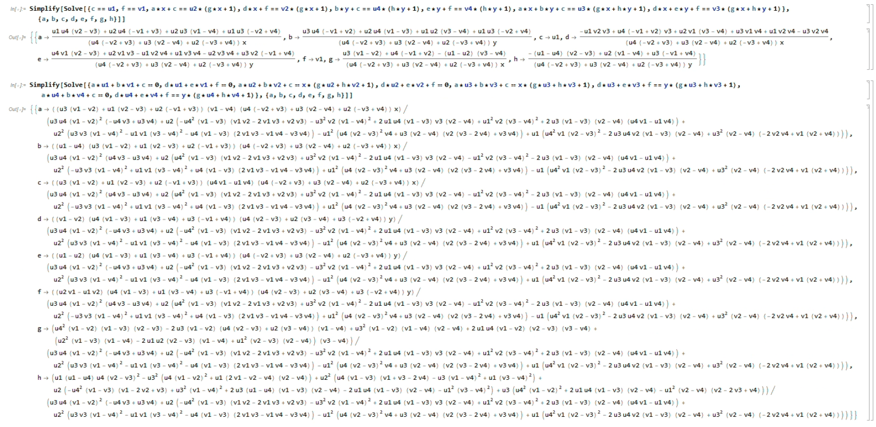
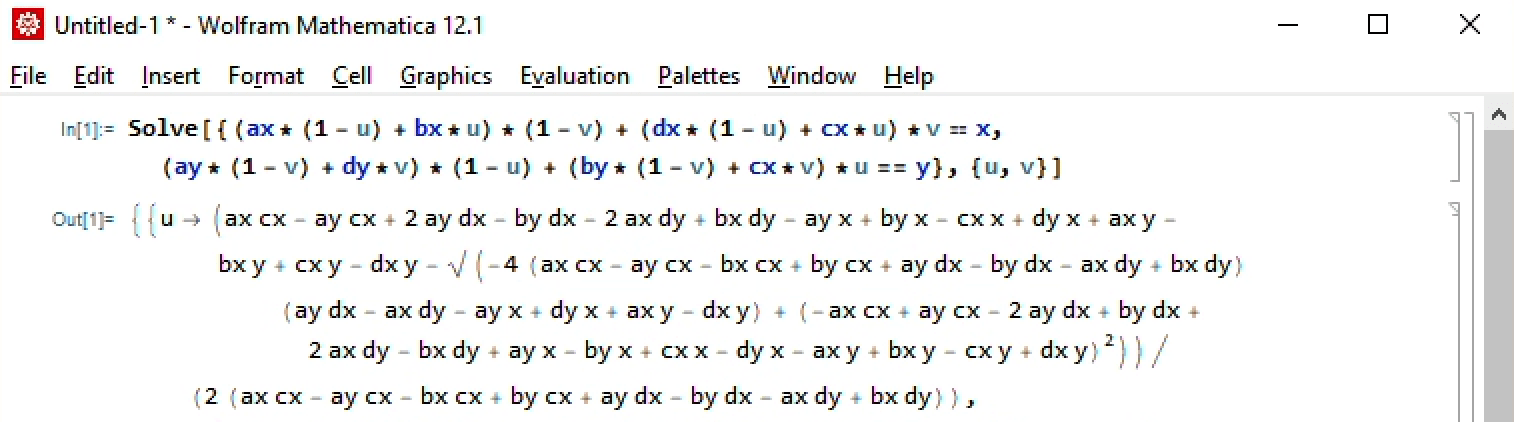
…and half a minute later, it got the answer! Here's a screenshot of the historic moment:

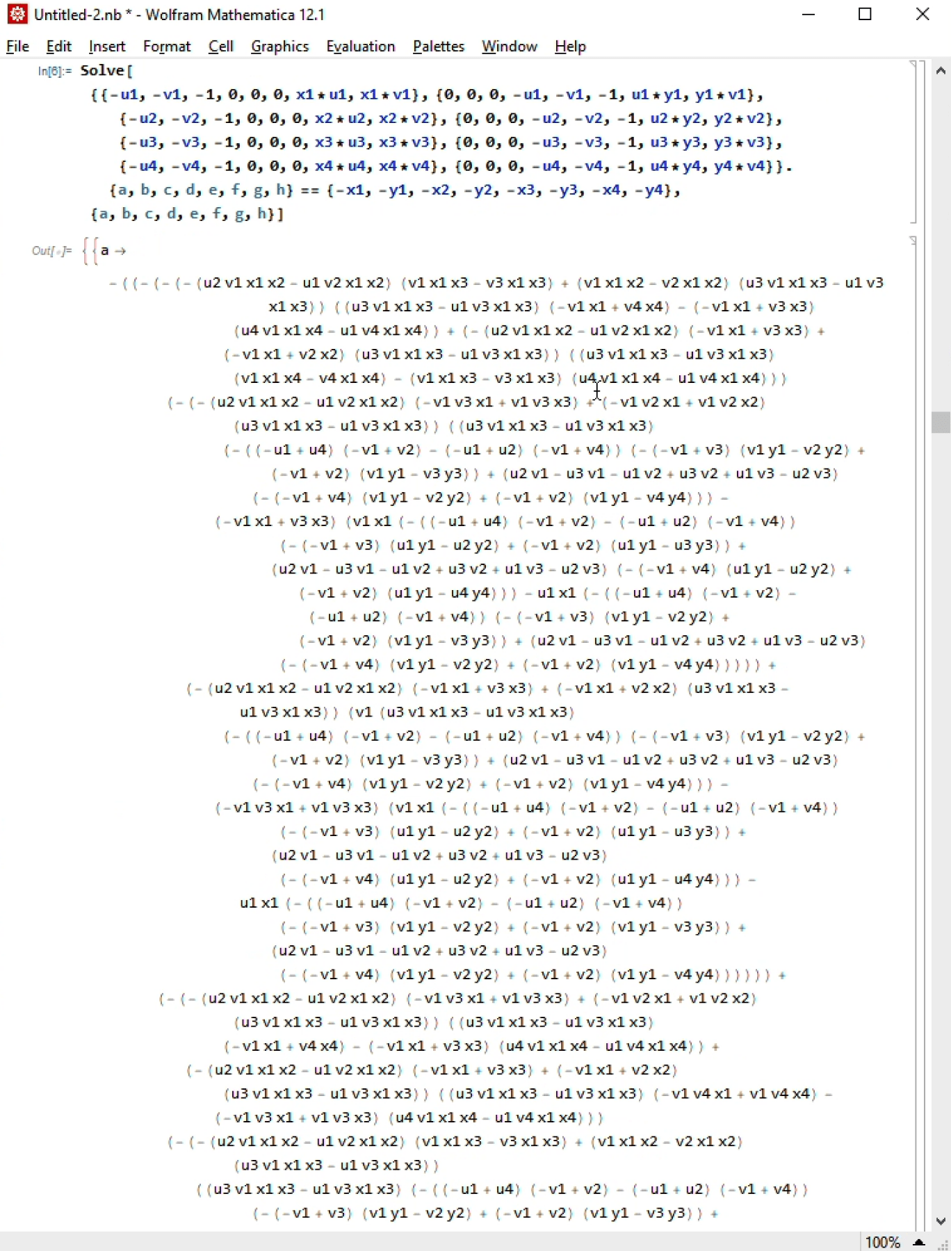
The only problem is, the solution is long. Like, really really long (just look at the position of that scrollbar!). If I copy it to a code file with max 80 char/line, it's 1400 lines long.

Time to Simplify!

Simplify[Out[1]]

It took two hours to complete, with intermittent complaints about how certain transformations timed out, and finally gave an answer 900 lines long. Still pretty long, but I'm willing to take it:

ExportString[Out[2],"Text"]

The full formula can be found in the source code.

My excitement hit a stone wall when I tested out this 900-line incantation in JavaScript:

console.log(a,b,c,d,e,f,g,h);

NaN NaN NaN NaN NaN NaN NaN NaN

Now, where in the 50,000 characters was the first NaN born…

Then I saw all the / signs in the formula, and it became immediately clear that zero divisions are near inevitable. Alas! Such is the bane of closed form expressions! But fear not, RNG to the rescue!

const EPS = 0.01;
x1 += (Math.random()-0.5)*2*EPS; y1 += (Math.random()-0.5)*2*EPS;
u1 += (Math.random()-0.5)*2*EPS; v1 += (Math.random()-0.5)*2*EPS;
x2 += (Math.random()-0.5)*2*EPS; y2 += (Math.random()-0.5)*2*EPS;
u2 += (Math.random()-0.5)*2*EPS; v2 += (Math.random()-0.5)*2*EPS;
x3 += (Math.random()-0.5)*2*EPS; y3 += (Math.random()-0.5)*2*EPS;
u3 += (Math.random()-0.5)*2*EPS; v3 += (Math.random()-0.5)*2*EPS;
x4 += (Math.random()-0.5)*2*EPS; y4 += (Math.random()-0.5)*2*EPS;
u4 += (Math.random()-0.5)*2*EPS; v4 += (Math.random()-0.5)*2*EPS;

Now the formula worked like a charm!

You might be wondering if there'd be any performance issues evaluating such a huge expression. Turns out that there'd be none. If I were to carry out the calculations by hand I'd probably need ten years, making a thousand mistakes and bored to death a million times in the process. But machines are built for stupid math like these! The entire matrix can be computed in less than a hot millisecond (node.js, MacBook Pro mid-2015)! Moreover it only needs to be computed per warp and NOT per pixel, so it can well be real time operation for reasonably-sized images.

Before we move on to code implementation, we would like to test if the special cases where either the source OR the destination quad is rectangular would make things significantly simpler. Turns out they are! Here're the systems and their solutions in Mathematica:

So if your use cases involves straightening up pictures or photoshopping 2D graphics onto images of 3D surfaces (which I imagine why image warping is needed anyways), give these formulae a shot!

Finally, I wrote a Processing demo to showcase how the magic formula can be used for image warping. Note that in Java and C/C++ etc., the datatype used in the calculation needs to be double(64-bit) instead of float (perhaps even better if there's long double), lest things overflow, and NaN strikes again!

You can find the unabridged source code here, but below are the key parts:

// disturbing vertices to prevent NaN's
float DBL_EPS = 0.0001;
double disturb(double x){
  double EPS = DBL_EPS;
  return x + Math.random()*EPS*2-EPS;
}

// compute Homography matrix by applying formula
float[] computeHMatrix(
  double x1,double y1,double x2,double y2,double x3,double y3,double x4,double y4,
  double u1,double v1,double u2,double v2,double u3,double v3,double u4,double v4
){
  x1 = disturb(x1); y1 = disturb(y1);
  x2 = disturb(x2); y2 = disturb(y2);
  x3 = disturb(x3); y3 = disturb(y3);
  x4 = disturb(x4); y4 = disturb(y4);
  u1 = disturb(u1); v1 = disturb(v1);
  u2 = disturb(u2); v2 = disturb(v2);
  u3 = disturb(u3); v3 = disturb(v3);
  u4 = disturb(u4); v4 = disturb(v4);

  double a = /* ... truncated */
  double b = /* ... truncated */
  double c = /* ... truncated */
  double d = /* ... truncated */
  double e = /* ... truncated */
  double f = /* ... truncated */
  double g = /* ... truncated */
  double h = /* ... truncated */

  return new float[]{(float)a,(float)b,(float)c,(float)d,(float)e,(float)f,(float)g,(float)h};
}

// apply Homography matrix via matrix multiplication
float[] applyHMatrix(float[] H, float u, float v){
  float x = H[0] * u + H[1] * v + H[2];
  float y = H[3] * u + H[4] * v + H[5];
  float z = H[6] * u + H[7] * v + 1;
  return new float[]{x/z,y/z};
}

// main routine to warp images with homogrphy
//+-----------------------------+ +-----------------------------+
//| (ax0,ay0) +-----+ (bx0,by0) | | (ax1,ay1) +-----+ (bx1,by1) |
//|           |      \          | |          /     /            |
//| (dx0,dy0) +-------+(cx0,cy0)| |(dx1,dy1)+-----+ (cx1,cy1)   |
//+-----------------------------+ +-----------------------------+
//               src             ->             dst
void warpHomographic(PImage src, PImage dst,
  float ax0, float ay0, float bx0, float by0, float cx0, float cy0, float dx0, float dy0,
  float ax1, float ay1, float bx1, float by1, float cx1, float cy1, float dx1, float dy1
){
  src.loadPixels();
  dst.loadPixels();
  float[] H = computeHMatrix(
    ax0,ay0,bx0,by0,cx0,cy0,dx0,dy0,
    ax1,ay1,bx1,by1,cx1,cy1,dx1,dy1
  );

  int[] roi = boundingBox(ax1,ay1,bx1,by1,cx1,cy1,dx1,dy1);
  for (int i = roi[1]; i <= roi[3]; i++){
    if (i < 0 || i > dst.height) continue;
    for (int j = roi[0]; j <= roi[2]; j++){
      if (j < 0 || j > dst.width) continue;

      if (!pointInQuad(j,i,ax1,ay1,bx1,by1,cx1,cy1,dx1,dy1)) continue;

      float[] xy = applyHMatrix(H, j, i);

      int val = sampler(src,xy[0],xy[1]);
      dst.pixels[i*dst.width+j] = val;
    }
  }
  dst.updatePixels();
}

Bilinear

The homographic method is all nice and good, but I was still left wondering if it's possible to use bilinear coordinates for warping (like the Pocket Handbook)?

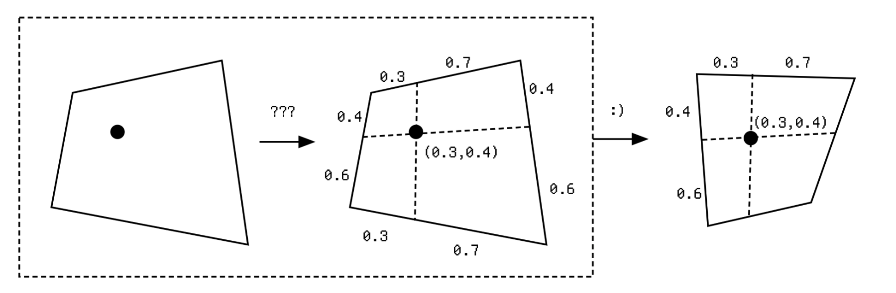
The key problem, which the book skipped (hence producing the aforementioned limitations), is how to convert Cartesian coordinates to bilinear coordinates. For it is easy to do the other way around from bilinear to Cartesian: simply apply it on a rectangle! But given an arbitrary point in space and an arbitrary quad, how can one describe the point's location in relation to the quad?

I drew inspiration from barycentric coordinates. Barycentric coordinates is the prevalent way in computer graphics to describe the position of a point in relation to a triangle $ABC$: If each vertex of the triangle is multiplied by a scalar weight and added together (say 20% of $A$ + 30% of $B$ and 50% of $C$), we get a point whose position is uniquely described by these weights.

Intuitively, the centroid is just 33.3% of $A$, 33.3% of $B$ and 33.3% of $C$. Thus we have the barycentric coordinates of the centroid as $(\frac{1}{3},\frac{1}{3})$. (The third $\frac{1}{3}$ can be implied from $1-\frac{1}{3}-\frac{1}{3}$). If we want the point to be closer to vertex $A$, then we can just add more weight to the first barycentric coordinate; and the same goes for the other two vertices.

Therefore, to compute barycentric coordinates $(u,v)$ from Cartesian $(x,y)$, one only needs to solve the following linear system:

So easy!

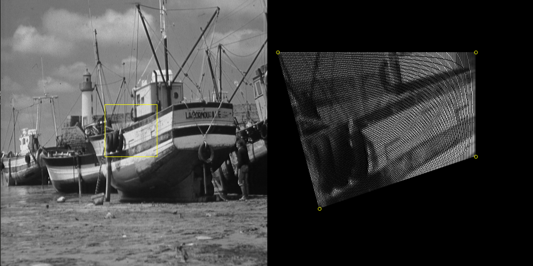
Now that we've seen how expressive barycentric coordinates are, the natural question to ask is: can we just use barycentric coordinates for quads too? After all, a quad is just two triangles placed together. We could apply warp to the upper-left triangle first, then the lower right. Would this reduction work?

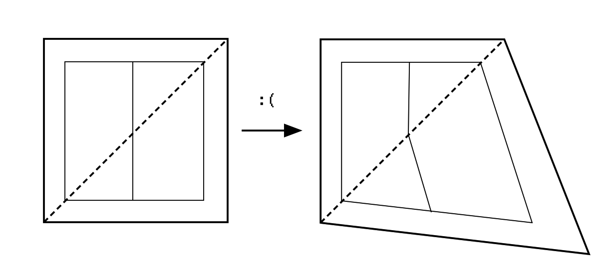
Unfortunately, as you can see in the illustration, our clever little scheme will fail miserably, as it'll break supposedly straight lines, and create discrepancy in stretching at different parts of image.

If you're thinking “Why do I care? as long as it fills all pixels in the quad…”, then barycentric coordinates is the perfect solution for you! You can also find an implementation for it in my source code for the project.

But things aren't that hard for the rest of us either: we can simply apply the idea behind finding barycentric coordinates, to derive a formula to find bilinear coordinates! A.K.A. solving systems of equations (yet again)!

We know that the expression for linear interpolation (lerp) is:

So that for bilinear interpolation is:

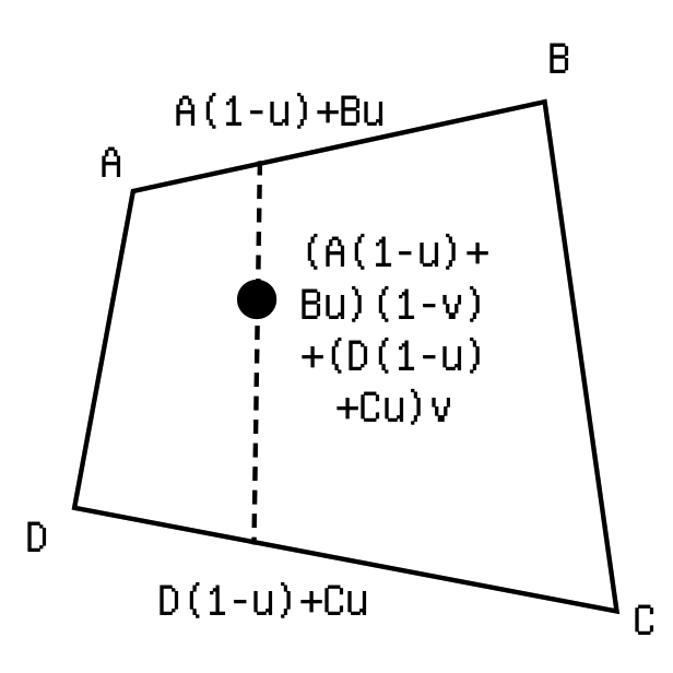
So to get $u$ and $v$ back, we need to solve the following system:

Now that system is not linear: notice how $v$ will be multiplied to $u$. Yet another reason to be lazy and ask Mathematica to do the dirty work!

Solve[{
  (ax*(1 - u) + bx*u)*(1 - v) + (dx*(1 - u) + cx*u)*v == y,
  (ay*(1 - v) + dy*v)*(1 - u) + (by*(1 - v) + cx*v)*u == x},
  {u,v}]

Mathematica thinks it's easy!

And after some copy-pasting and wrapping, we can obtain this Java code: (Notice how we still need to disturb the vertices, lest there be NaN's):

float[] cart2quad(
  float x,float y,
  float ax,float ay,
  float bx,float by,
  float cx,float cy,
  float dx,float dy){

   x = disturb( x);  y = disturb( y);
  ax = disturb(ax); ay = disturb(ay);
  bx = disturb(bx); by = disturb(by);
  cx = disturb(cx); cy = disturb(cy);
  dx = disturb(dx); dy = disturb(dy);

  float u = (ay*cx - ax*cy - 2*ay*dx + by*dx + 2*ax*dy - bx*dy + ay*x - 
  by*x + cy*x - dy*x - ax*y + bx*y - cx*y + dx*y + sqrt(pow(by*dx - bx*dy 
  - by*x + cy*x - dy*x + ay*(cx - 2*dx + x) + bx*y - cx*y + dx*y - 
  ax*(cy - 2*dy + y),2) + 4*(ay*(cx - dx) + by*(-cx + dx) - (ax - 
  bx)*(cy - dy))*(ay*(dx - x) + dy*x - dx*y + ax*(-dy + 
  y))))/(2*(ay*(cx - dx) + by*(-cx + dx) - (ax - bx)*(cy - dy)));

  float v = (2*ay*bx - 2*ax*by - ay*cx + ax*cy + by*dx - bx*dy - ay*x + by*x - 
  cy*x + dy*x + ax*y - bx*y + cx*y - dx*y + sqrt(pow(by*dx - bx*dy - by*x 
  + cy*x - dy*x + ay*(cx - 2*dx + x) + bx*y - cx*y + dx*y - ax*(cy - 
  2*dy + y),2) + 4*(ay*(cx - dx) + by*(-cx + dx) - (ax - bx)*(cy - 
  dy))*(ay*(dx - x) + dy*x - dx*y + ax*(-dy + y))))/(2*(ay*(bx - cx) + 
  ax*(-by + cy) + by*dx - cy*dx - bx*dy + cx*dy));

  return new float[]{u,v};
}

Since unlike Homography, whose matrix needs only be pre-computed once, we need to find the bilinear coordinate for every pixel in the target quad and map back to cartesian coordinate in the source quad, we would like to optimize the function a little bit, by caching invariants that can be pre-calculated.

Having no idea what each term means and solely by staring at the formula to identify similarities, I was able to dissect the calculation into this, considerably reducing duplicate work:

// pre-calculate params invariant to pixel coordinate
float[] cart2quadParams(
  float ax,float ay,
  float bx,float by,
  float cx,float cy,
  float dx,float dy
){

  float n = by*dx-bx*dy;
  float k = 2* ((ay*(cx - dx) + by*(-cx + dx) - (ax - bx)*(cy - dy)));
  float d = (2*(ay*(bx - cx) + ax*(-by + cy) + by*dx - cy*dx - bx*dy + cx*dy));
  float s = ax-bx+cx-dx;
  float r = ay-by+cy-dy;

  if (k == 0 || d == 0){
    float EPS = 0.01;
    if (k == 0){
      cx -= EPS;
      ax -= EPS;
      cy -= EPS;
    }else{
      bx -= EPS;
      by -= EPS;
    }
    return cart2quadParams(ax,ay,bx,by,cx,cy,dx,dy);
  }

  return new float[]{ax,ay,bx,by,cx,cy,dx,dy,n,k,d,s,r};
}

// calculate bilinear coordinates from pre-calced params
float[] cart2quadFromParams(float x,float y,float[]P){

  float ax = P[0], ay = P[1], bx = P[2], by = P[3], cx = P[4], cy = P[5];
  float dx = P[6], dy = P[7], n = P[8], k = P[9], d = P[10], s = P[11], r = P[12];

  r *= x;
  s *= y;

  float f = n + r + ay*(cx - 2*dx) - s - ax*(cy - 2*dy);
  float t = sqrt(f*f + 2*k*(ay*(dx - x) + dy*x - dx*y + ax*(-dy + y)));
  float m = r - s;
  float q = n + t;
  float u = (ay*cx - ax*cy - 2*ay*dx + 2*ax*dy + q + m)/k;
  float v = (2*ay*bx - 2*ax*by - ay*cx + ax*cy + q - m)/d;

  return new float[]{u,v};
}

Notice that another nice improvement is that we no longer need to disturb the vertices (randomly that is), since we can pinpoint the terms that cause denominators to become 0, and purposefully nudge only these variables slightly.

With the trivial bilinear-to-Cartesian transformation implemented:

float[] quad2cart(
  float u,float v,
  float ax,float ay, float bx,float by,
  float cx,float cy, float dx,float dy){
  float x = (ax*(1-u)+bx*u)*(1-v)+(dx*(1-u)+cx*u)*v;
  float y = (ay*(1-v)+dy*v)*(1-u)+(by*(1-v)+cy*v)*u;
  return new float[]{x,y};
}

The main bilinear warp routine can look something like this:

void warpQuadcentric(PImage src, PImage dst,
  float ax0, float ay0, float bx0, float by0, float cx0, float cy0, float dx0, float dy0,
  float ax1, float ay1, float bx1, float by1, float cx1, float cy1, float dx1, float dy1
){
  src.loadPixels();
  dst.loadPixels();
  int[] roi = quadRoi(ax1,ay1,bx1,by1,cx1,cy1,dx1,dy1);
  float[] P = cart2quadParams(ax1,ay1,bx1,by1,cx1,cy1,dx1,dy1);
  for (int i = roi[1]; i <= roi[3]; i++){
    if (i < 0 || i > dst.height) continue;
    for (int j = roi[0]; j <= roi[2]; j++){

      if (j < 0 || j > dst.width) continue;
      //float[] uv = cart2quad(j,i,ax1,ay1,bx1,by1,cx1,cy1,dx1,dy1);
      float[] uv = cart2quadFromParams(j,i,P);

      if (Float.isNaN(uv[0]) || Float.isNaN(uv[1]) || uv[0] < 0 || uv[0] > 1 || uv[1] < 0 || uv[1] > 1) continue;
      float[] xy = quad2cart(uv[0],uv[1],ax0,ay0,bx0,by0,cx0,cy0,dx0,dy0);
      int val = sampler(src,xy[0],xy[1]);
      dst.pixels[i*dst.width+j] = val;
    }
  }
  dst.updatePixels();
}

The unabridged implementation can again be found in the source code.

Biangular

While working on the Homographic and Bilinear methods, I gradually start to recall that I've actually solved the problem of image warping once before, in one of my older projects.

Digging out the old code, I discovered that I was using a method quite distinct from the two! Though not as performant (as it involves trigonometric functions), the idea was quite interesting, and could be worthy of sharing. Maybe one day I or someone else will be able to find a performant implementation for it, who knows!

Upon closer inspection, I think the name Biangular befits this coordinate system. Here is how it works:

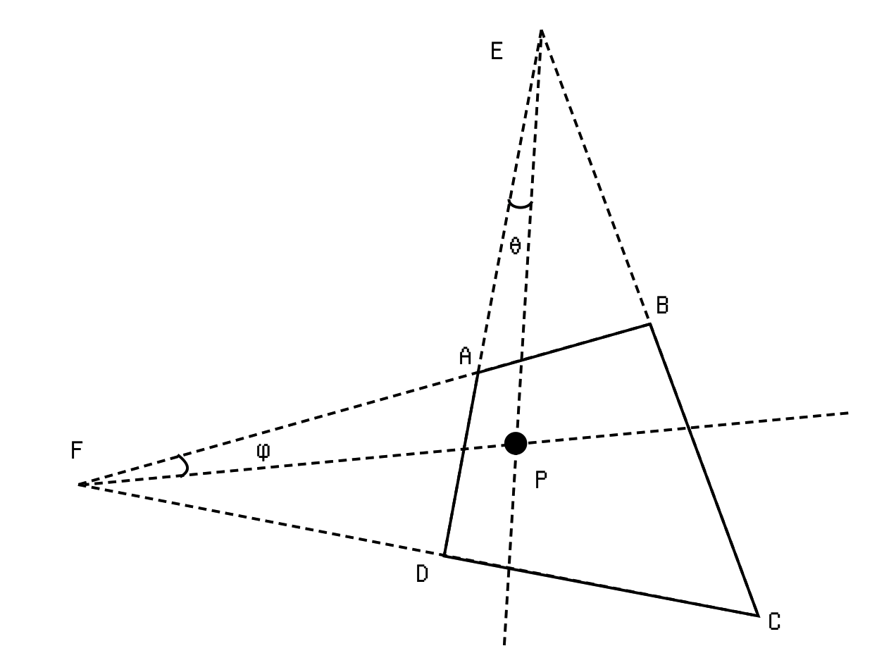
Given a quad $ABCD$ with no parallel edges (assume this is the general non-degenerate case) find an intersection between $AD$ and $BC$, as well as one between $AB$ and $CD$. Label them $E$ and $F$. Find the vector pointing from $E$ to our coordinate in question $P$, and compute the angle between that vector and $\vec{EA}$. Divide the angle by $\angle AEB$ to get a fraction ($\frac{\angle AEP}{\angle AEB}$) describing the first component of the biangular coordinate. The second component can be similarly computed as a ratio between the angles $\frac{\angle AFP}{\angle AFD}$.

If there're parallel edges, instead compute the ratio between the distance from the point to one edge, and the distance between the edges. This works because $\tan(x)\approx x$ as $x \to 0$.

To transform from biangular back to Cartesian, we can compute the intersection between the ray fixed by $F$ and $\frac{\angle AFP}{\angle AFD}$, and the ray fixed by $E$ and $\frac{\angle AEP}{\angle AEB}$ to get $P$.

(As you can see I used to be a rather geometry-centred problem-solver before being spoiled by linear algebra.)

My old implementation of this algorithm doesn't look too efficient or robust from the eyes of now-(hopefully)-smarter me, and only contains the forward transformation, so I thought I'd redo it proper. Here's the new version:

float cart2sweep(
  float x,float y,
  float ax,float ay,
  float dx,float dy,
  float ang,
  float D,
  float[]isect){
  if (isect == null){
    return pointDistanceToLine(x,y,ax,ay,dx,dy)/D;
  }
  float vx = x-isect[0];
  float vy = y-isect[1];

  float A = vecAngle(dx-isect[0],dy-isect[1],vx,vy);

  return A/ang;
}

float[] sweep2cart(
  float u, float v,
  float ax, float ay, float bx, float by,
  float cx, float cy, float dx, float dy,
  float angV,float angH,
  float[] isectV, float[] isectH
){
  float l0x, l0y, l1x, l1y;
  float m0x, m0y, m1x, m1y;

  if (isectV != null){
    float dax = dx-ax;
    float day = dy-ay;
    float au = u*angV;
    float[] urxy = vecRot(dax,day,au);
    l0x = isectV[0];
    l0y = isectV[1];
    l1x = l0x+urxy[0];
    l1y = l0y+urxy[1];
  }else{
    l0x = ax * (1-u) + bx * u;
    l0y = ay * (1-u) + by * u;
    l1x = dx * (1-u) + cx * u;
    l1y = dy * (1-u) + cy * u;
  }

  if (isectH != null){
    float bax = bx-ax;
    float bay = by-ay;
    float av = v*angH;
    float[] vrxy = vecRot(bax,bay,av);
    m0x = isectH[0];
    m0y = isectH[1];
    m1x = m0x+vrxy[0];
    m1y = m0y+vrxy[1];
  }else{
    m0x = ax * (1-v) + dx * v;
    m0y = ay * (1-v) + dy * v;
    m1x = bx * (1-v) + cx * v;
    m1y = by * (1-v) + cy * v;
  }
  return lineIntersect(l0x,l0y,l1x,l1y,m0x,m0y,m1x,m1y);
}

void warpSweep(PImage src, PImage dst,
  float ax0, float ay0, float bx0, float by0, float cx0, float cy0, float dx0, float dy0,
  float ax1, float ay1, float bx1, float by1, float cx1, float cy1, float dx1, float dy1
){
  src.loadPixels();
  dst.loadPixels();

  float[] isectV0 = lineIntersect(ax0,ay0,dx0,dy0, bx0,by0,cx0,cy0);
  float[] isectH0 = lineIntersect(ax0,ay0,bx0,by0, dx0,dy0,cx0,cy0);
  float[] isectV1 = lineIntersect(ax1,ay1,dx1,dy1, bx1,by1,cx1,cy1);
  float[] isectH1 = lineIntersect(ax1,ay1,bx1,by1, dx1,dy1,cx1,cy1);

  float d1_tb=0, d1_lr=0;
  if (isectV1 == null) d1_lr = pointDistanceToLine(ax1,ay1,bx1,by1,cx1,cy1);
  if (isectH1 == null) d1_tb = pointDistanceToLine(ax1,ay1,dx1,dy1,cx1,cy1);

  float angV0=0, angH0=0, angV1=0, angH1=0;

  if (isectV0 != null) angV0 = vecAngle(dx0-isectV0[0],dy0-isectV0[1], cx0-isectV0[0],cy0-isectV0[1]);
  if (isectH0 != null) angH0 = vecAngle(ax0-isectH0[0],ay0-isectH0[1], dx0-isectH0[0],dy0-isectH0[1]);
  if (isectV1 != null) angV1 = vecAngle(dx1-isectV1[0],dy1-isectV1[1], cx1-isectV1[0],cy1-isectV1[1]);
  if (isectH1 != null) angH1 = vecAngle(ax1-isectH1[0],ay1-isectH1[1], dx1-isectH1[0],dy1-isectH1[1]);


  int[] roi = quadRoi(ax1,ay1,bx1,by1,cx1,cy1,dx1,dy1);
  for (int i = roi[1]; i <= roi[3]; i++){
    if (i < 0 || i > dst.height) continue;
    for (int j = roi[0]; j <= roi[2]; j++){
      if (j < 0 || j > dst.width) continue;
      if (!pointInQuad(j,i,ax1,ay1,bx1,by1,cx1,cy1,dx1,dy1)) continue;

      float u = cart2sweep(j,i,ax1,ay1,dx1,dy1,angV1,d1_lr,isectV1);
      float v = cart2sweep(j,i,bx1,by1,ax1,ay1,angH1,d1_tb,isectH1);

      float[] xy = sweep2cart(u,v,ax0,ay0,bx0,by0,cx0,cy0,dx0,dy0,angV0,angH0,isectV0,isectH0);

      int val = sampler(src,xy[0],xy[1]);
      dst.pixels[i*dst.width+j] = val;
    }
  }
  dst.updatePixels();
}

The code above calls to several helper functions such as lineIntersect, pointDistanceToLine, vecAngle(angle between 2 vectors) and vecRot(rotate vector by angle), which can be found in the full source for the project.

As you can see it's quite a chore to implement, and doesn't offer any particular nice property to choose it over homography or bilinear. But I hope you find it no less fun!

Anyways, that concludes our fun adventure with image warping functions for now. Check out the source code!