$- x^4 + x^3 + x^2$

2021/03/04

A while back when I was working on a project at STUDIO for Creative Inquiry, one interesting little problem that I came across is to find a shaping function for a zooming interaction.

Say that you're using the “pinch to zoom” gesture on an image. We wanted the image to be a bit “lazy” in changing from its default scale. If you only twitched your finger ever so slightly, the image barely enlarges (or shrinks). As your gesture becomes more significant, the image catches up with the specified zooming factor.

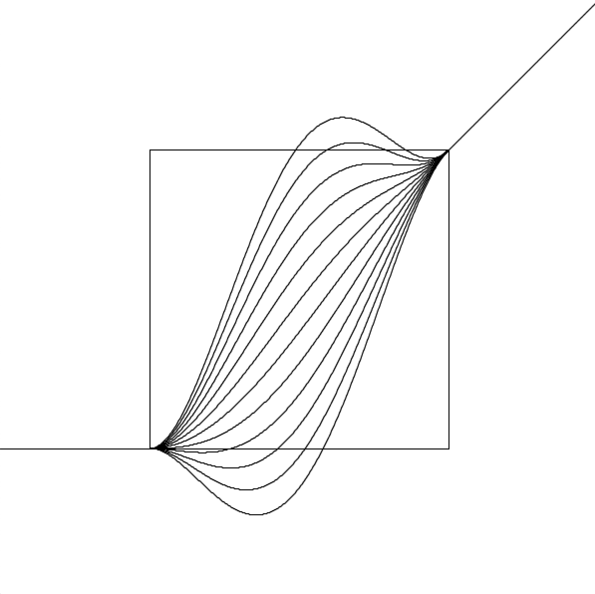
In other words, If 1.0 is the default scale, we would like a shaping function that is tangent to $y=1$ at $x=1$, and tangent to $y=x$ at $x=1\pm r$ where $r$ is a constant, as shown in the illustration below:

Notice the flat “seat” in the middle, and the exact 45° diagonal behavior at either ends.

Because of its symmetrical properties, it is equivalent to the easier alternative of finding a function tangent to $y=0$ at $x=0$ and tangent to $y=x$ at $y=1$.

One solution is of course to use a cubic Bézier curve: place the two control points to specify the tangent, like how they're doing it in CSS. However, since Bézier is parametric and I require a $y=f(x)$ expression instead, I'll have to interpolate between samples on the Bézier, or use Newton's method to solve $t$ for $x$, both of which could be a juggle between smoothness, efficiency and simplicity, so I wanted to look for non-parametric alternatives first.

My first thought back then was to round up “the usual suspects”: $x^2$, $x^3$, $sin(x)$, $e^x$… With some scaling and translation, one of them gotta do the trick!

Unfortunately, the main catch is that, when you scale a function along the x or y axis independently, its derivative is undesirably squashed too, and vice versa. (Try with $x^3$ for example).

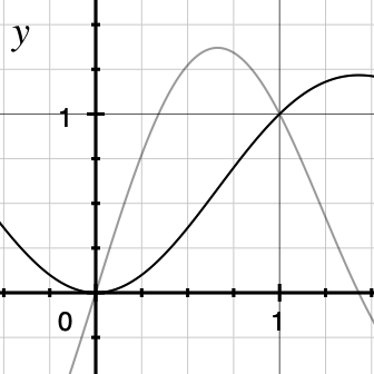
Though there's actually at least one widely known function that does just the correct thing ($1-\frac{\sin(\pi x)}{\pi x}$, otherwise known as Lanczos or sinc, see below for its graph with derivative in gray), I wasn't aware of this property of it at the time.

The “quick and dirty” hack I pulled up then was to use blending. Because basically, all we want is something that looks like $y=x^2$ or $y=x^3$ near the zero, and something like $y=x$ near one. Why not create a chimera with lion head of $y=x^3$ and snake tail of $y=x$, and use blending function make a mush of the middle?

With linear interpolation it would be:

//0 <= x <= 1
float t = x;
float y = pow(x,3) * (1-t) + x * t;

I ended up using a sinusoidal posed as a sigmoid for the blending, as it looked the nicest for my use case:

//0 <= x <= 1
float t = cos(PI*x+PI)/2 + 1/2;
float y = pow(x,3) * (1-t) + x * t;

And this was my final implementation, padding and transforming the function for the aforementioned context of zooming images:

float inertiaScalingFunction(float x, float r){ 
  // 0 <= x < inf, 0 < r < 1
  if (1-r < x && x < 1+r){ // non-linear part
    x = (x-(1-r))/(r*2); // normalize x
    float y =  (0.5 + 0.5*pow((x-a)/0.5, 3.0));
    // blending function
    float t =  1.0/2-cos(2*PI*x)/2;
    float w = y*t+x*(1-t); // blend with linear
    return 1-r+w*r*2; // denormalize and return
  }
  return x; // linear part
}

The additional r parameter allows specifying the size of the flat “seat” at $x=1$.

Back then my problem was solved, and I really didn't give it a second thought and moved on.

But more recently the notion bubbled up in my mind that there should be a systematic way to find truckloads of functions with these desired properties, and I decided to take a closer look.

First, consider the simpler linearly interpolated version:

Since $t=x$ it can be simplified to:

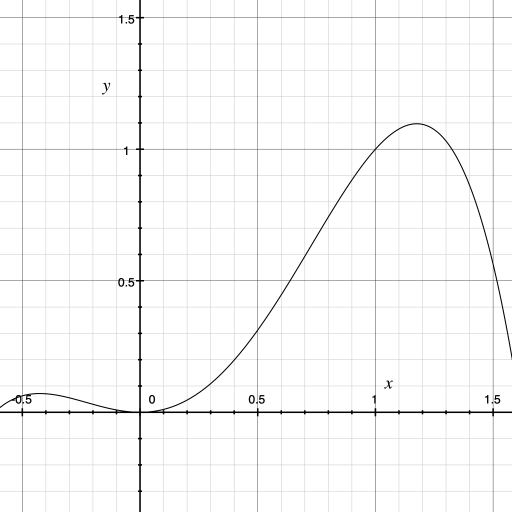
Plotting the polynomial we see that it seems to behave as expected for $0\leq x\leq 1$:

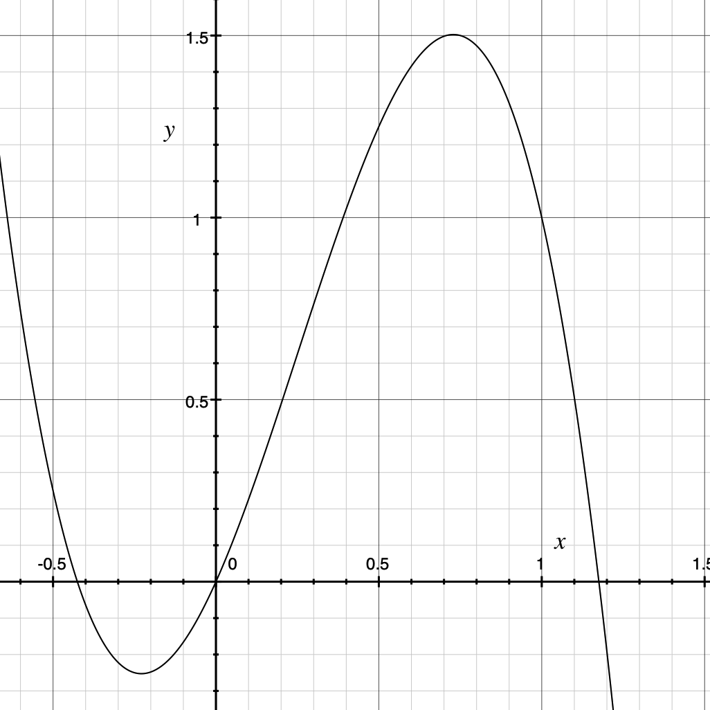
To verify, we calculate its derivative:

Plot:

At this point a nice approach to the solution becomes very apparent: $- x^4 + x^3 + x^2$ is a polynomial. Recall that polynomials are awesome, and as long as you're willing to go higher order it can bend to whatever shape you want! (Think Taylor series). Therefore we just need to solve a system of equations to determine the coefficients for potentially eligible polynomials.

The equations are dead simple:

Let's start with an order of 4 first, to honour the order of the first polynomial I found to satisfy the equations.

Let

Therefore

So the system becomes:

Kick the zeros out:

This means that for the 4th order, we have one “free” coefficient, and the other two can be solved accordingly. It also means that there's a single solution for the cubic version, and 0 solutions for the quadratic.

Apply grade school knowledge to solve for $b$ and $c$:

Substitute $a=0$, we find the single solution for cubic:

Plot:

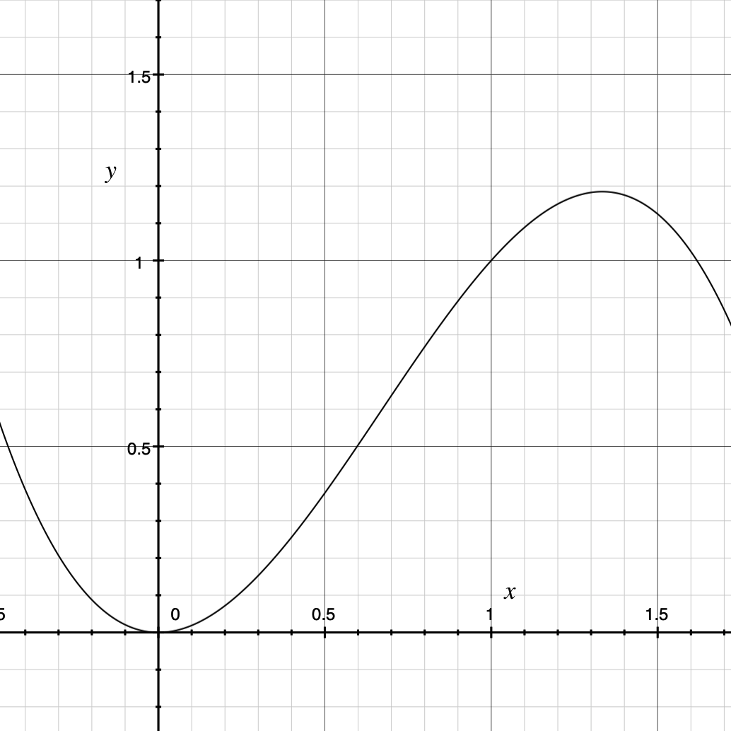
We can also verify that our first set of coefficients (-1,1,1,0,0) satisfies this system:

Now let's get back to coding to explore the space of the 4th order coefficient $a$, using Processing for visualization:

void order4(){
  int n = 50;
  float m = 12;
  int w = 300;
  translate((width-w)/2,(height-w)/2);
  rect(0,0,w,w);

  for (int i = 0; i < n; i++){
    float a = map(i,0,n,-m,m);
    float b = - 2 * a - 1;
    float c = a + 2;
    //println(a,b,c);
    beginShape();
    for (int j = 0; j < w; j++){
      float x = (float)j/(float)w;
      float y = a * x * x * x * x + b * x * x * x + c * x * x;

      vertex(j,w-y*w);
    }
    endShape();
  }
}
void setup(){
  size(600,600);
  noFill();
}
void draw(){
  background(255);
  order4();
}

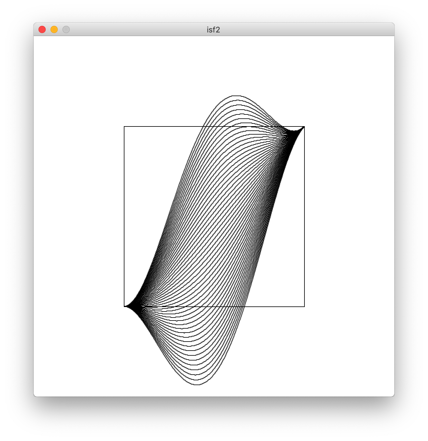
As you can see all the curves satisfy the properties we ever wanted. How nice!

Now we can give 5th order a shot:

Let

The system:

Solve for $c$ and $d$:

This time for the visualization, we use the mouseX coordinate for $a$ and the iterative loop for $b$, so we can clearly see the effect of each:

void order5(){
  int n = 12;
  float ma = 10;
  float mb = 10;
  int w = 300;
  translate((width-w)/2,(height-w)/2);
  rect(0,0,w,w);

  for (int i = 0; i < n; i++){

    float a = map(constrain((float)mouseX/width,0,1),0,1,-ma,ma);
    float b = map(i,0,n,-mb,mb);
    float c = -1 - 3 * a - 2 * b;
    float d = 2 * a + b + 2;
    //println(a,b,c,d);
    beginShape();
    for (int j = 0; j < w; j++){
      float x = (float)j/(float)w;
      float y = a * x * x * x * x * x + b * x * x * x * x + c * x * x * x + d * x * x;
      vertex(j,w-y*w);
    }
    endShape();
  }
}

We can go to even higher order, but I'm bored.

Instead, let's go back to the first stage:

//0 <= x <= 1
float t = x;
float y = pow(x,3) * (1-t) + x * t;

We had $x^3$ for the chimera head. Would that generalize to $x^4$, or even $x^n$?

Therefore

Indeed! We have

How nice! But what about $2x^n$ or even $kx^n$? The problem apparently becomes solving for $k$ in $f(1)=-k+1+1=1$, and the only solution is $k=1$.

However if we use the cosine-based blending mentioned earlier, no matter what we choose for the head, it seems to work regardless:

Say we plot the graph with $k=9$ and $n=7$. Marvel at how it's almost not going to work when the function is getting close to $x=1$, but the $\cos$ blending function is so powerful that it brings a plot twist, and just manages to get the derivative back to $1$ at $x=1$.

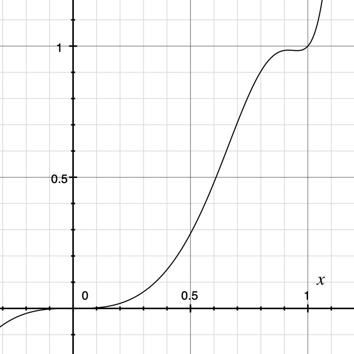
Intuitively, I think the blending function need to have a zero derivative at $x=1$ for this to work for any head function, which the $\cos$ satisfies. Time to prove it!

Let the blending function be $b(x)$ and the head function be $h(x)$, we have:

Therefore

And the following system needs to be satisfied:

Now using the two obvious facts about $h(x)$ (i.e. $h(0)=0$ and $h'(0)=0$), we solve for $b(x)$, to see what properties it needs to satisfy:

The first three equations too simple, and the fourth too complicated! Let's assume that $b(1)=1$, which is what we usually expect of a blending function, and see what happens:

We can observe that:

In other words, we either need the blending function to be flat at $x=1$, or we need the head function to pass through $(1,1)$. Which is pretty consistent with our observations so far: with $h(x)=x^n$ we satisfying the latter, while $b(x)=\frac{\cos( x\pi -\pi)+1}{2}$ the former!

So another possible class of blending function besides the $\cos$ one that could work by satisfying $b'(1)=0$ is:

For example, the graph of $y=\left( x-9x^{7} \right)\left( \left( x-1 \right)^{3}+1 \right)+9x^{7}$:

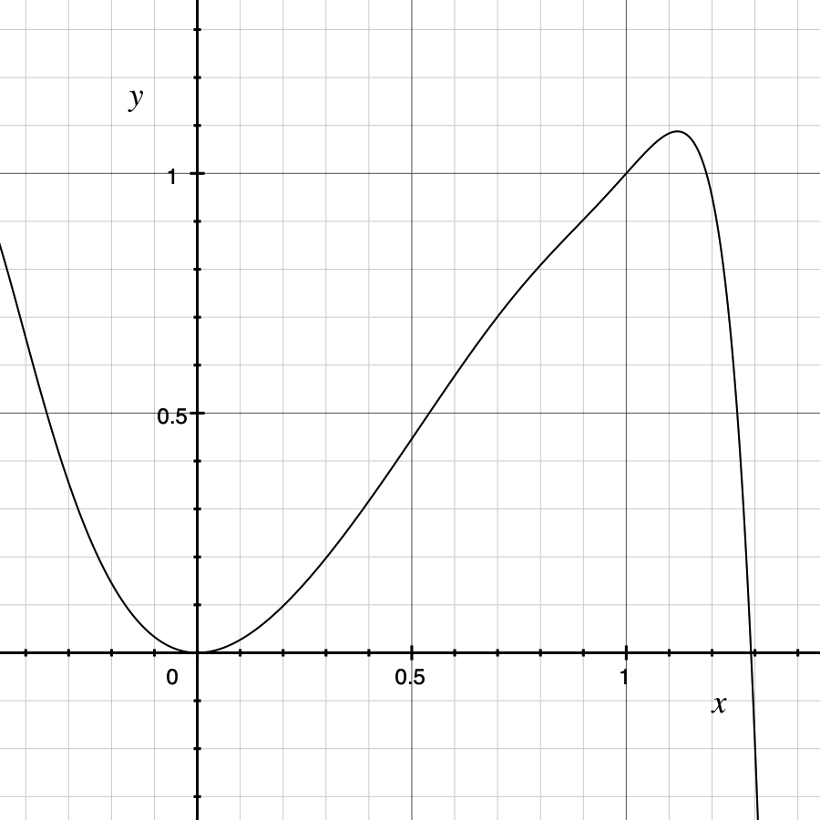
What's even more fun, is that according to the rules, we can even do away with $h(x)$ altogether, by setting it to $h(x)=0$. Let's see:

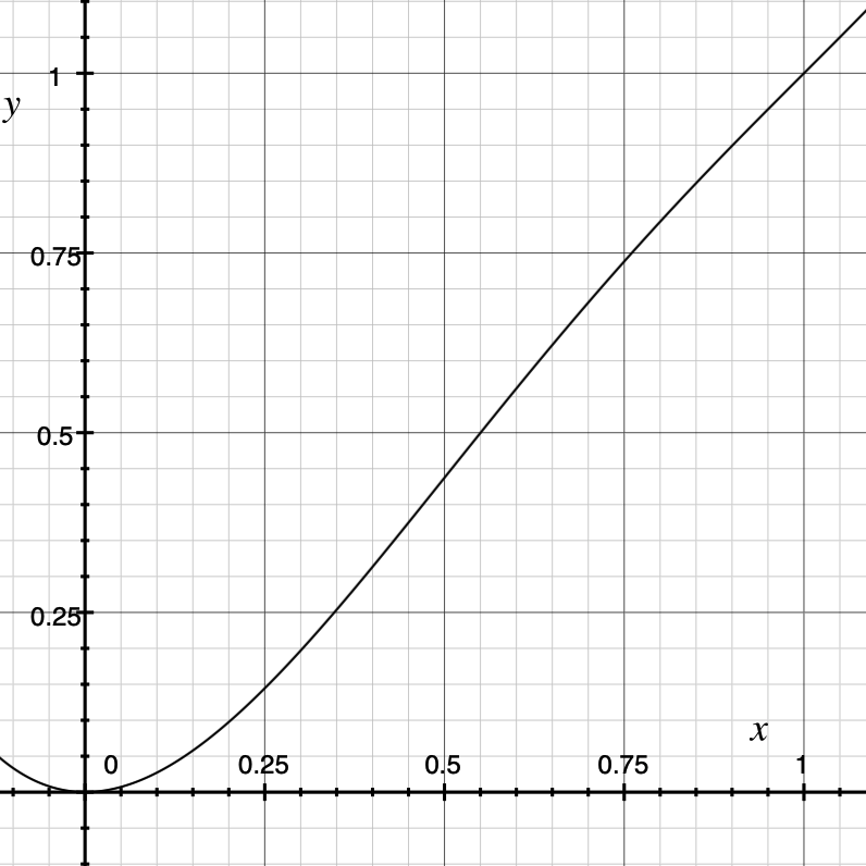
And yep, it totally works! This means that we can just grab any function that passes through $(0,0)$ and $(1,1)$ and has a derivative of 0 at $(1,1)$, multiply that by $x$, and get the inertial scaling function we want!

Now expanding the polynomial above, we get

Remember our earlier formula for polynomials of degree 4:

Which checks out. Cool! Just for fun, here're some more neat ones I constructed with this method:

As you can see it all comes down to just starting from any function with a stationary point or extrema, scale it to fit into the range [0,1], and slap an $x\cdot$ before it. You can let your imagination run wild.

For example, if we start with the cosh function:

We mirror (about x axis), translate (y by 2) and scale (x by its root, $\ln(2+\sqrt{3})$) the function so that it passes through (0,0), and the minima (now maxima) is at (1,1):

After simplification:

Multiply by $x$:

…and we get yet another function that fits our criteria. Unlike our previous polynomial method, which can only lead to, well, polynomials, this new method works for all sorts.

Finally, if we're somehow smart enough to come up with this $b(x)$:

(Verifying that $b(0)=b'(1)=0$ and $b(1)=1$), we would've discovered the aforementioned Lanczos function:

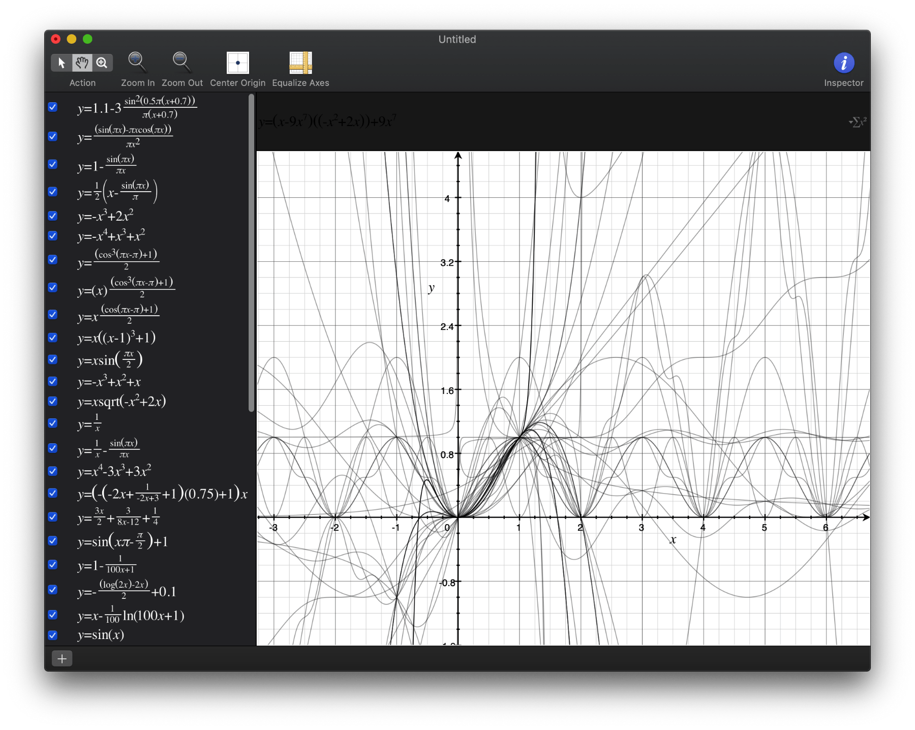
In this short experiment I mainly explored two possible approaches to generating the “inertia scaling function”, one is by modelling it directly with a polynomial and solving a system of equations for the coefficients, and the other by breaking it down to two easier problems of finding a function that satisfies the required behavior near $x=0$ and another blending function to interpolate it with $y=x$ toward $x=1$.

Perhaps from the perspective of a maths person, my polynomial adventure is nothing but a silly rant that leads to trivial facts, but it sure did keep my little brain entertained for a bit!

If you enjoy weird shaping functions, be sure to check out Pattern Master by Golan Levin (it includes the aforementioned Lanczos window and Newton's method for solving Bézier curves) as well as p5.func by R. Luke DuBois.